Signal Processing & Wavelets

Introduction

Wavelets are powerful oscilatory functions that can behave as a basis for several functions in the \(L^2\) space. The primary motivations for the development of wavelets as tool for signal analysis arises from the inability of the complex exponentials in the fourier series to form a basis for non-periodic functions. The capabilty of wavelets to perform multi-resolution analysis has lead to wavelet theory being used in several digital signal processing applications including medical imaging, communication systems, speech processing and machine learning.

This article is based on the Wavelets course offered by Dr.Subrahmanya Sastry Challa .

Fourier Series

The Fourier Series formulation was given by the French Mathematician Joseph Fourier to the solve the heat equation. \[ \frac{\partial T}{\partial t} = D\frac{\partial^2 T}{\partial x^2} \] Where \(T\) is the temperature at a given point and time and \(D\) is the diffusivity constant.

The Fourier Series representation of a periodic function \(f\) with period \(l\) can be expressed as a sum of scaled complex exponentials where \(f\in L^2[-l,l]\). \[ \begin{equation} f(x)=\sum_{\small{n=-\infty}}^{\small{\infty}} c_n.e^{j\frac{2\pi}{l}nx} \end{equation} \]

The expression for \(c_n\) can be evaluated as

\[ c_n = \frac{1}{2l}\int_{-l}^{l} f(x).e^{-j\frac{2\pi}{l}nx}dx \]

import numpy as np
import matplotlib.pyplot as plt
x = np.linspace(-7, 7, 1000)
A = 1  # Amplitude
def square_wave(x,T):
    return A*np.where(np.mod(x,T) < T/2, 1, -1)
T = 2*np.pi
def fourier_series(x, n_terms):
    result = np.zeros_like(x)
    for n in range(1, 2*(n_terms + 1)): #
        if n % 2 == 1:  # Only odd harmonics contribute to the square wave
            result += (1/(n)) * np.sin((n)*x)
    return A * (4/np.pi) * result
N=[1,5]
plt.figure(figsize=(5, 2.5))
for n in N:
    plt.plot(x, fourier_series(x, n), label=f'{n} Terms')
plt.plot(x, square_wave(x,T), label='Square Wave')
# plt.title('Fourier Series Approximation of a Square Wave')
plt.xlabel('x')
plt.ylabel('f(x)')
# plt.legend('upper right')
# plt.grid()
plt.axis('off')
plt.tight_layout()
plt.show()

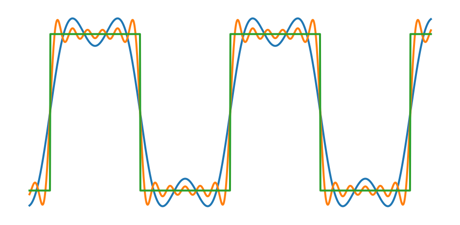
Figure 1: Fourier Series approximation of a square wave

We can observe that upon increasing the number of fourier coefficients \(c_n\) the signal approaches the orignal signal. The fourier coefficients can be thought of strength of oscilatory frequency components \(w=\frac{2\pi n}{l}\).

What is interesting to note is that the entire basis of the function space \(L^2[-l,l]\) arises from a single orthogonal basis \(e^{\left(j\frac{2\pi}{l}x\right)^n}\) where \(n\in \mathbb{Z}\). This lead to work in the direction if there exists such class of function which can form a basis for the entire \(L^2\) space.

Fourier Transform

The fourier transform extends the idea of fourier series for aperiodic functions by formulating the a periodic functions as periodic function with infinite period(not very rigorous but I’ll let it be).

The function \(f(x)\) can be expressed as \[ f(x)=\sum_{\small{n=-\infty}}^{\small{\infty}} \left(\int_{-l}^{l} \frac{1}{2l}f(\tau).e^{-jw_0n\tau}d\tau \right)e^{jw_0nx} \] where \(w_0=\Delta w =\frac{2\pi}{2l}\) as lim \(l\rightarrow \infty \therefore l=\frac{\pi}{\Delta w}\) and \(nw_0=w\)

This can then be solved as

\[ f(x)=\frac{1}{2\pi}\int_{-\infty}^{{\infty}} \left(\int_{-\infty}^{\infty} f(\tau).e^{-jw\tau}d\tau \right)e^{jwx} \]

Where the inner integral represents the Fourier Transform : \[ \hat{f}(w)=\int_{\mathbb{R}}f(x).e^{-jwx}dx \]

The existence of the Fourier Transform is constraint by the Dirichlet conditions which is that \(f\) is absolutely integrable, i.e.

\[ \int_{\mathbb{R}} |f(x)| dx < \infty \]

When \(f\) is discrete represented as \(f[x]\) , the dicrete analog of the Fourier Transform or the Fast Fourier Transform Algorithm is used, which was developed by Cooley–Tukey.The story for the development of this algorithm is pretty interesting and can be found in this article by iflscience.

Another Interesting propery assoiciated with the fourier is the conversation of energy of the energy in time and frequency domain, this can be put down as

\[ \int_{\mathbb{R}} |f(x)|^2dx=\int_{\mathbb{R}}|\hat{f}(w)|^2dw \]

import numpy as np
import matplotlib.pyplot as plt
# fourier of a cosine wave
x = np.linspace(-10, 10, 1000)
f = [0.5,1,2.5]  # Frequency of the cosine wave
signal = 0.5*np.cos(2 * np.pi * f[0] * x) +0.75*np.cos(2 * np.pi * f[1] * x) +0.2*np.cos(2 * np.pi * f[2] * x)
# Compute the Fourier Transform
fourier_transform = np.fft.fft(signal)
#0.02 is the sampling interval which is the difference between two consecutive x values
# the max frequency is half the sampling rate =50/2 = 25 Hz
# difference between two frequencies is 1/(N*dt)=1/T=1/20 where N is the number of samples and dt is the sampling interval
frequencies = np.fft.fftfreq(len(signal), d=(x[1] - x[0]))
plt.figure(figsize=(5, 2.5)) 
plt.plot(frequencies, np.abs(fourier_transform))
# plt.title('Fourier Transform')
plt.xlim(-3, 3)
plt.axis('off')
plt.tight_layout()
plt.show()

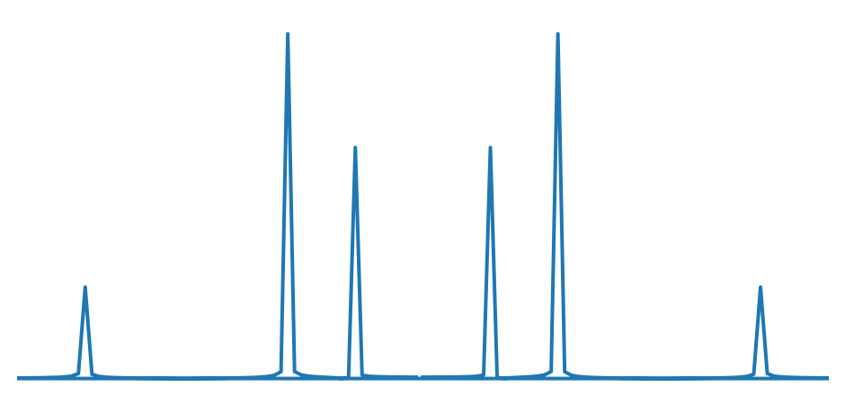
Figure 2: Fourier Transform of a Cosine Wave with frequency 0.5,1,2.5 Hz mixed together in thr ratio 0.5:0.75:0.2

We can see from the above plot, the Fourier Transform of the signal has three peaks at the frequencies of the cosine waves that were mixed together. The height of the peaks corresponds to the amplitude of the respective cosine waves in the original signal. Although the abilty to resolve time-frequency information is lost in the Fourier Transform, the Short-Time Fourier Transform was provided as an solution for this problem.

Short Time Fourier Transform

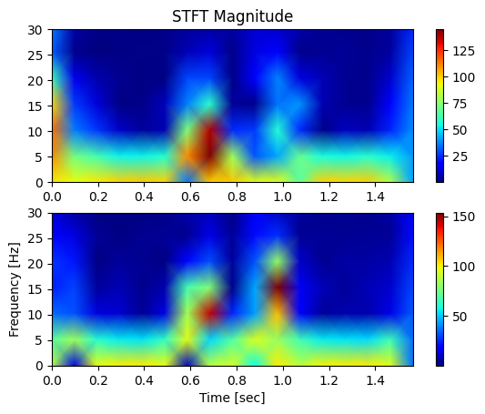
The Short Time Fourier Transform applies the fourier transform in a section of the signal by utilizing a shifting window, this can be expressed as: \[ \hat{f}(b,w) = \int_{\mathbb{R}} f(x)\overline{w(x-b)}e^{-jwx}dx \] This is an example of STFT computation from a ECoG signal, which is a invasive methodology for neural signal extraction.

STFT of neural signal obtained for showing a person a object (top) and STFT of obtained upon showing a person a face (bottom)

What is specifically interesting here that cognition of be represented as different frequency components in the brain !!

We can observe that the alpha (5-10 Hz) beta-band frequency(15-20 Hz) is particularly higher in case of the STFT where the subject was shown the face and these peaks in the alpha beta frequency correspond to the time the face was shown and removed. Thus showing humans have a greator cognitive salience associated with faces than objects.

In the case of the Short-Time Fourier Transform, the window size is fixed. We need a small window to resolve the time of high frequency burst but require a longer window to detect a low frequency signal. Hence the requirement is to construct a variable window which can transform such that the window size is small for high frequency components and large for low frequency components. This is where wavelets come into the picture.

Wavelets

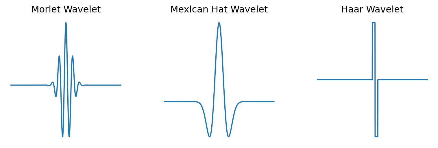
Wavelets are finitely supported oscillatory functions that can give rise to daughter wavelets by translation and scale modulation.

The daughter wavelets \(\psi_{ab}\) can be represented as the following function of the mother wavelet \(\psi\) \[ \psi_{ab}=\frac{1}{\sqrt{a}}\psi \left(\frac{x-b}{a} \right) \] The continuous wavelet can be defined as an operator acting upon \(f\), \[ T_{\psi}f(a,b)=\int_{\mathbb{R}} f(x)\overline{\psi_{ab}(x)}dx=\dot \langle f,\psi_{ab} \rangle \] The admissible wavelet for which wavelet transform is such that it satifies the condition for the admissable constant \(C_{\psi}\) \[ C_{\psi}=\int_{\mathbb{R}}\frac{|\hat{\psi}(w)|^2}{w}dw < \infty \]

For \(C_{\psi}\) to exist

\[ \hat{\psi}(0)=\int_{\mathbb{R}} \psi(x)dx = 0 \]

Which implies that wavelets behave like a high-pass filter attenutating the frequencies in the lower frequencies.

import numpy as np
import matplotlib.pyplot as plt
x = np.linspace(-10, 10, 1000)
# Morlet wavelet
def morlet_wavelet(x, sigma=1):
    return np.exp(-x**2 / (2 * sigma**2)) * np.cos(5 * x)
# Mexican Hat wavelet
def mexican_hat_wavelet(x):
    return (1 - x**2) * np.exp(-x**2 / 2)
# Haar wavelet
def haar_wavelet(x):
    return np.where((x >= 0) & (x < 0.5), 1, np.where((x >= 0.5) & (x < 1), -1, 0))
plt.figure(figsize=(8, 3))
plt.subplot(1, 3, 1)
plt.plot(x, morlet_wavelet(x))
plt.title('Morlet Wavelet')
plt.axis('off')
plt.subplot(1, 3, 2)
plt.plot(x, mexican_hat_wavelet(x))
plt.title('Mexican Hat Wavelet')
plt.axis('off')
plt.subplot(1, 3, 3)
plt.plot(x, haar_wavelet(x))
plt.title('Haar Wavelet')
plt.tight_layout()
plt.axis('off')
plt.show()

Figure 3: Wavelet functions: Morlet, Mexican Hat and Haar wavelets

The Inverse wavelet transform can be expressed as:

\[ f(x)=\frac{1}{C_{\psi}}\int_{\mathbb{R}}\int_{\mathbb{R}} T_{\psi}f(a,b)\overline{\psi_{ab}(x)}\frac{dadb}{a^2} \]

We can’t have \(a\) and \(b\) taking continuous values for a computational implementation and thus require discretized representation for them. Here is where we utilize the discrete wavelet transform.

Discrete Wavelet Transform

The discrete wavelet \(\psi_{[m,n]}\) is represented by the discrete scale and translation factors, \(a=a_0^m\) and \(b=nb_0a_0^m\) , where \(a_0\) and \(b_0\) are fixed parameters and \(m,n\in \mathbb{Z}\).

Thus the set of wavelets is defined as :

\[ \psi_{[m,n]}=a_0^{-m/2}\psi(a_0^{-m}x-nb_0) \]

The discrete wavelet transform can be expressed as: \[ T_{\psi}f(m,n)=\int_{\mathbb{R}} f(x)\overline{\psi_{[m,n]}(x)}dx \]

If the set of wavelets \(\psi_{[m,n]}\) forms an frame for \(L^2(\mathbb{R})\) then \(f\) can be represented as a linear combination of the wavelets : \[ f(x)=\sum_{m,n} d_{m,n}\psi_{[m,n]}(x) \]

If the set of wavelets \(\psi_{[m,n]}\) forms an orthonormal basis for \(L^2(\mathbb{R})\) then the coefficients \(d_{m,n}\) can be evaluated as follows: \[ d_{m,n}=\int_{\mathbb{R}} f(x)\overline{\psi_{[m,n]}(x)}dx=\langle f,\psi_{[m,n]} \rangle \]

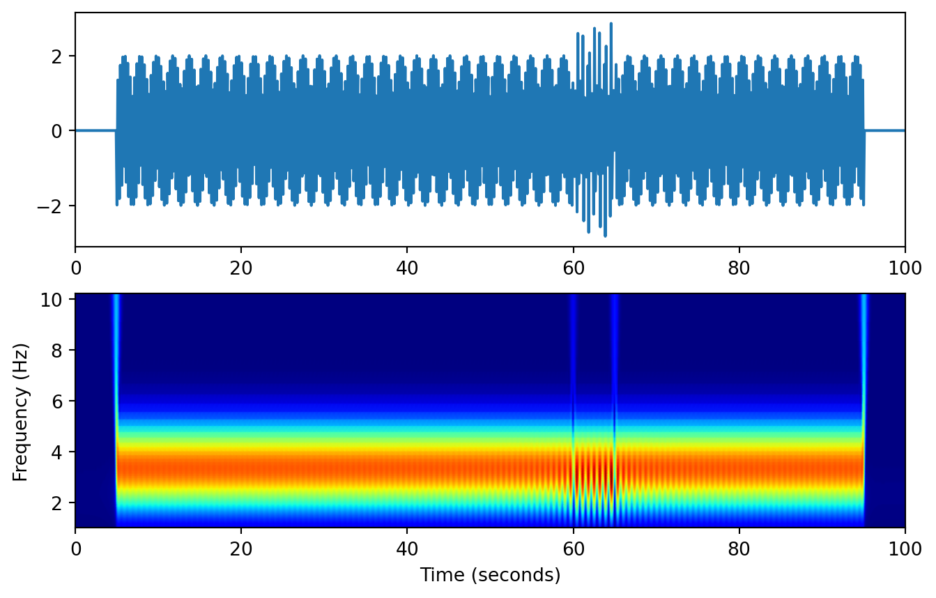
import numpy as np
import matplotlib.pyplot as plt
from spkit.cwt import ScalogramCWT

# 1. Setup Signal
x = np.linspace(0, 100, 1000)  # Time vector from 0 to 100 seconds
# Signal 1: 50 Hz (20-40s), Signal 2: 30 Hz (60-80s)
signal = np.where((x > 5) & (x < 95), 2*np.cos(2 * np.pi * 3.5 * x), 0) + \
         np.where((x > 60) & (x < 65), 2*np.cos(2 * np.pi * 5 * x), 0)
fs = 1 / (x[1] - x[0])

# 2. Compute CWT
# PlotScaling=False to avoid double plotting
XW, S = ScalogramCWT(signal,x, fs=fs, wavelet='morlet', n_scales=512, plotPSD=True)

# 3. Correct Frequency Mapping
freqs = fs / S 

# 4. Use pcolormesh for accurate physical units
plt.figure(figsize=(8, 5))

# Normalize for visibility
# XW_abs = np.abs(XW) / np.max(np.abs(XW))
# extent = [x[0], x[-1], freqs[0], freqs[-1]]
# pcolormesh handles the non-linear frequency spacing of CWT perfectly
# plot orignal signal
plt.subplot(2, 1, 1)
# start from 0 to 100 seconds currently there is a lot of empty space in the beginning and end of the signal which is not very informative, so we can zoom in on the relevant time range
plt.plot(x, signal, label='Signal')
plt.xlim(0, 100)
# start from 0 to 100 seconds

# plt.xlabel("Time (seconds)")
# remove y
# plt.ylabel("Amplitude")
# plt.title("Original Signal")

plt.subplot(2, 1, 2)
plt.pcolormesh(x, freqs, np.abs(XW), shading='gouraud', cmap='jet')

plt.xlabel("Time (seconds)")
plt.ylabel("Frequency (Hz)")

# Zoom in on the relevant frequency range
plt.ylim(1, 10.2) 
# plt.colorbar(label="Normalized Magnitude")
plt.show()

Figure 4: Orignal signal (top) and its Discrete Wavelet Transform (bottom)

Frame Theory

A frame collection \(\{\phi\}_{i\in J}\) is defined in the hibert space \(\mathcal{H}\) that satisfies the following property \[ A\left\lVert f\right\rVert^2_2 \leq \sum_{i \in J}\left\lVert \langle f,\phi_i\rangle \right\rVert^2 \leq B\left\lVert f\right\rVert^2_2 \forall f\in \mathcal{H} \]

If \(A=B\) then the frame is a tight frame.

For a collection \(\{\phi\}_{i\in J}\) satisfying the above property we define the Frame operator \(F:\mathcal{H}\rightarrow l^2(J)\)

\[ Ff=\{\langle f,\phi_i\rangle\}_{i\in J} \]

We define the adjoint operator \(F^*:l^2(J)\rightarrow H\)

\[ SF^*{c_i}=\sum_{i\in J}c_i\phi_i \]

The self adjoint operator \(S=F^*F:\mathcal{H}\rightarrow \mathcal{H}\) can be defined as

\[ Sf=F^*Ff=\sum_{i\in J}\langle f,\phi_i\rangle \phi_i \]

The frame property can be equivalently written as \[ A\langle f,f \rangle\leq \langle Sf,f\rangle \leq B\langle f,f \rangle \]

For a tight frame we have \(S=AI_d\) and thus the inverse of the frame operator can be computed as \(S^{-1}=\frac{1}{A}I_d\).

\[ f=\frac{1}{A}\sum_{i\in J}\langle f,\phi_i\rangle \phi_i \]

When the frame is not tight we define the dual frame \(\{\tilde{\phi}_i\}_{i\in J}\) as

\[ \tilde{\phi}_i=S^{-1}\phi_i \]

Thus the signal can be reconstructed as

\[ f=\sum_{i\in J}\langle f,\tilde{\phi}_i\rangle \phi_i=\sum_{i\in J}\langle f,\phi_i\rangle \tilde{\phi}_i \]

Frames provide an interesting approach to represent a signal wherein frames that do not form basis have a non-trivial null space.Thus a signal can have multiple representation from the same frame.

\(S^{-1}\) can be computed numerically using the von Neumann series as

\[ S^{-1}=\frac{2}{A+B}\sum_{n=0}^{\infty} R^n \]

where \(R=I-\frac{2}{A+B}S\) and the series converges if \(\left\lVert R \right\rVert < 1\) which is satisfied for any frame collection.

Orthogonal Wavelet

When \({\psi}\) is frame in the dual frame in frequency domain can be defined as \[ {\tilde{\psi}}(w)=\frac{\hat{\psi}(w)}{\sum_{k \in \mathbb{Z}}|\hat{\psi(w+w\pi k)|^2}} \] For a orthogonal wavelet the dual frame is the same as the original frame hence the condition for an orthogonal wavelet can be expressed as \[ \sum_{k \in \mathbb{Z}}|\hat{\psi(w+w\pi k)|^2}=1 \forall w \in \mathbb{R} \]

Multiresolution Analysis

The multiresolution analysis is a sequence of closed subspaces \(V_j\) of \(L^2(\mathbb{R})\) such that

1. \(V_{-1} \subset V_{0} \subset V_{1} \dots\)
2. \(V_{j\in \mathbb{Z}}\) is dense is \(L^2(\mathbb{R})\)
3. \(\cap V_{j}=\{0\}\)
4. \(f \in V_j \implies f(2x) \in V_{j+1}\)
5. There exists a function \(\phi \in V_0\) such that \(\{\phi(x-k)\}_{k\in \mathbb{Z}}\) is an orthonormal basis for \(V_0\).

We can define the wavelet space \(W_j\) as the orthogonal complement of \(V_j\) in \(V_{j+1}\), i.e. \(V_{j+1}=V_j \oplus W_j\). The wavelet function \(\psi\) can be defined as the function in \(W_0\) such that \(\{\psi(x-k)\}_{k\in \mathbb{Z}}\) is an orthonormal basis for \(W_0\).

# drawing the multiresolution analysis spheres V0, V1 and V2 as spheres of radius 1, 0.5 and 0.25 respectively centered at the origin in a 3D space
import plotly.graph_objects as go
import numpy as np

def create_interactive_spheres():
    fig = go.Figure()

    radii = [1, 0.5, 0.25]
    names = ["Low Res (Scale 1)", "Mid Res (Scale 2)", "High Res (Scale 3)"]
    colorscale = ['Purples', 'Magenta', 'thermal']

    for i, (r, name) in enumerate(zip(radii, names)):
        # Generate sphere coordinates
        u = np.linspace(0, 2 * np.pi, 50)
        v = np.linspace(0, np.pi, 50)
        x = r * np.outer(np.cos(u), np.sin(v))
        y = r * np.outer(np.sin(u), np.sin(v))
        z = r * np.outer(np.ones(np.size(u)), np.cos(v))

        fig.add_trace(go.Surface(x=x, y=y, z=z, 
                                 opacity=0.7 - (i*0.05), 
                                 name=name,
                                 showscale=False,
                                 colorscale=colorscale[i]))

    fig.update_layout(
        title='Interactive Multiresolution Analysis',
        scene=dict(
            xaxis=dict(visible=False),
            yaxis=dict(visible=False),
            zaxis=dict(visible=False),
            aspectmode='data'
        ),
        margin=dict(l=0, r=0, b=0, t=40)
    )
    fig.show()

create_interactive_spheres()

Figure 5: Multiresolution analysis spheres

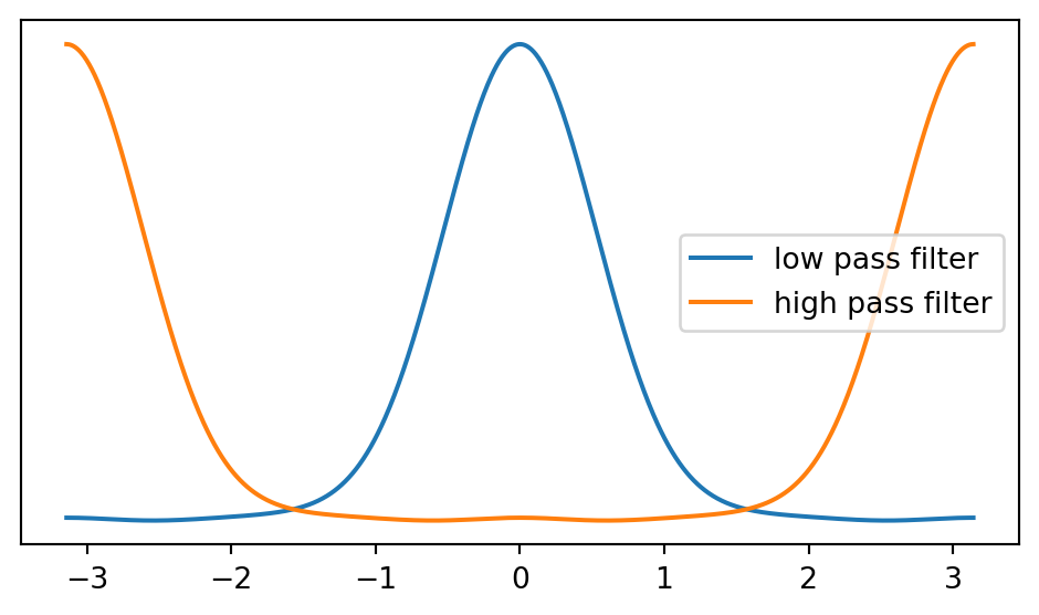
We know \(\phi \in V_0 \subset V_1\) \[ \phi(x)=\sum_{k \in \mathbb{Z}} h_k \phi(2x-k) \] This can be expressed in the frequency domain as \[ \hat{\phi}(w)=m_0\left(\frac{w}{2}\right)\hat{\phi}\left(\frac{w}{2}\right) \] where \(m_0(w)=\frac{1}{\sqrt{2}}\sum_{k \in \mathbb{Z}} h_k e^{-jkw}\) is the low pass filter associated with the scaling function \(\phi\).

Similarly we can express the two scale relation for the wavelet function \(\psi\) as \[ \psi(x)=\sum_{k \in \mathbb{Z}} g_k \phi(2x-k) \] This can be expressed in the frequency domain as \[ \hat{\psi}(w)=m_1\left(\frac{w}{2}\right)\hat{\phi}\left(\frac{w}{2}\right) \] where \(m_1(w)=\frac{1}{\sqrt{2}}\sum_{k \in \mathbb{Z}} g_k e^{-jkw}\) is the high pass filter associated with the wavelet function \(\psi\).

Using the two scale relation for the scaling function \(\phi\) we can express \(\hat{\phi}(w)\) as \[ \hat{\phi}(w)=\prod_{j=1}^{\infty} m_0\left(\frac{w}{2^j}\right)\hat{\phi}(0) \] where \(\hat{\phi}(0)=1\)

The low pass and high pass filter satisfy the following condition. \[ |m_0(w)|^2 + |m_0(w+\pi)|^2 = 1 \] The relation between the low pass coefficients \(h_k\) and the high pass coefficients \(g_k\) for a \(N\) coeffiecient wavelet can be expressed as \[ g_k = (-1)^k h_{N-1-k} \]

import numpy as np
import matplotlib.pyplot as plt
import math
w = np.linspace(-np.pi, np.pi, 1000)
# h_k=h-k

hk=[0.125, 0.25, 0.75, 1, 0.75, 0.25, 0.125]
map_hk=[-3,-2,-1,0,1,2,3]
map_gk=[-1,0,1,2,3,4,5]
gk=[(-1)**map_gk[k]*hk[len(hk)-1-k] for k in range(len(hk))]
print(gk)
m0 = np.zeros_like(w, dtype=complex)
m1 = np.zeros_like(w, dtype=complex)
m0pi = np.zeros_like(w, dtype=complex)
for k in range(len(hk)):
    m0 += hk[k] * np.exp(-1j * map_hk[k] * w)
    m1 += gk[k] * np.exp(-1j * map_gk[k] * w)
    m0pi+= hk[k] * np.exp(-1j * map_hk[k] * (w + np.pi))
plt.figure(figsize=(5, 3))
plt.plot(w, np.abs(m0)**2, label='low pass filter')
plt.plot(w, np.abs(m1)**2, label='high pass filter')
# plt.plot(w, np.abs(m0pi)**2+np.abs(m0)**2, label='low pass filter shifted by pi')
# plt.plot(w, np.abs(m0)**2 + np.abs(m1)**2, label='sum of low and high pass filters')
plt.plot    
plt.yticks([])
plt.tight_layout()
# legend in upper right
plt.legend()
plt.show()

[-0.125, 0.25, -0.75, 1, -0.75, 0.25, -0.125]

Figure 6: Low pass and High pass filter

Decomposition Reconstruction Algorithm

From the MRA frameworkthe function \(f \in L^2(\mathbb{R})\), there exist a sclae \(J\) such that \(f_J \approx f\). The function \(f_J\) can be expressed as a linear combination of the scaling functions \(\phi_{j,k}\) at scale \(J\) and translation \(k\) as follows: \[ f_J = \sum_{k \in \mathbb{Z}} c_{j,k} \phi_{j,k} \] Therefore the coefficients \(c_{j,k}\) can be computed as the inner product of the function \(f\) with the scaling function \(\phi_{j,k}\) due to the orthonormality property of the scaling function \(\phi_{j,k}\) : \[ c_{j,k} = \langle f, \phi_{j,k} \rangle \]

These coefficients can be computed using the two scale relation for the scaling function \(\phi\) using the MRA property that \(\phi \in V_0 \subset V_1\) as follows: \[ \langle f, \phi_{j,k} \rangle = \sum_{n \in \mathbb{Z}} h_n \langle f, \phi_{j+1,2k+n} \rangle \] \[ c_{j,k} = \sum_{n \in \mathbb{Z}} h_n c_{j+1,2k+n} \]

This can be represented as a convultion operation of the signal with the low pass filter \(h_n\) followed by downsampling by a factor of 2 i.e \[ c_{j,k} = (h_n * c_{j+1,n})\downarrow 2 \]

Similarly for the wavelet coefficients \(d_{j,k}\) we can express them as a convolution operation of the signal with the high pass filter \(g_n\) followed by downsampling by a factor of 2 i.e \[ d_{j,k} = (g_n * c_{j+1,n})\downarrow 2 \]

\[ c_{j+1,n} \;\longrightarrow\; \begin{cases} \ast\,h_n \;\longrightarrow\; \downarrow 2 \;\longrightarrow\; c_{j,k} \\[4pt] \ast\,g_n \;\longrightarrow\; \downarrow 2 \;\longrightarrow\; d_{j,k} \end{cases} \] The reconstruction of the signal can be expressed as an upsampling operation of the coefficients \(c_{j,k}\) and \(d_{j,k}\) followed by a convolution operation with the low pass filter \(h_n\) and high pass filter \(g_n\) respectively i.e \[ c_{j+1,n} = (h_n * c_{j,k})\uparrow 2 + (g_n * d_{j,k})\uparrow 2 \] \[ d_{j,k} \;\longrightarrow\; \uparrow 2 \;\longrightarrow\; \ast\,g_n \;\longrightarrow\; c_{j+1,n} \] This decomposition and reconstruction algorithm is the basis for the fast wavelet transform algorithm which is used in several applications including image compression, denoising and feature extraction where the input data is represented as the scaling coefficient at the highest scale .

Applications of Wavelets

Wavelets are used in several applications including image compression, denoising and feature extraction. The most popular application of wavelets is in image compression where the JPEG2000 standard uses wavelet transform for image compression. There are also interesting applications in medical imaging in compressive sensing for fast MR reconstruction and in the analysis of neural signals for feature extraction.

Feature extraction for deep learning applications have also recently gained popularity. Fundamental grounding in wavelets and frame theory was provided by Dr. Daubechies in her book Ten Lectures on Wavelets.

Overall a fascinating field grounded in strong fundamental theory and with several applications in signal processing and machine learning.

---

This page is made using Quarto see https://quarto.org.